Note

You can download this example as a Jupyter notebook or start it in interactive mode.

Power Portfolio Build-Out Example

This notebook provides a simplified example of building a power generation portfolio using linopy. The goal is to demonstrate the process of setting up and solving a linear optimization problem where different power generation resources are selected and built to meet future energy demands.

import matplotlib.pyplot as plt
import numpy as np
import pandas as pd
import xarray as xr

import linopy as lp

Problem Statement

This notebook presents an example portfolio expansion model used to meet an energy need. This was originally developed for a hydropower utility. Hydropower utilities can be energy limited (i.e., monthly energy balance) rather than capacity limited (i.e., hourly generating capacity), therefore, this algorithm addresses a monthly energy need rather than an hourly capacity need. A different algorithm would be needed to meet capacity needs and would include battery storage, etc.

This notebook addresses the question: what is the least-cost way to meet an energy need in the future?

Generate Dummy Data

The following cells only generate synthetic input data for the example. You can skim them and focus on the linopy model, which is defined further below. ### Energy Need

This analysis assumes that an energy need has been identified through modeling and simulation. For this example, we will assume the energy need is as follows:

def generate_dummy_energy_needs(start_year=2024, years=10):
    # Generate a monthly date range
    dates = pd.date_range(start=f"{start_year}-01-01", periods=years * 12, freq="ME")

    # Create a sinusoidal pattern for energy needs with a downward trend over time
    months = np.arange(len(dates))

    # Base seasonal pattern using sine functions (with phase shift for winter, spring, etc.)
    seasonal_pattern = np.sin(
        2 * np.pi * (months % 12) / 12
    )  # Basic seasonal pattern (positive in spring/fall, negative in winter/summer)

    # Adjust the pattern so that winter months trend more negative over time
    winter_weight = 0.5 * (
        np.cos(2 * np.pi * (months % 12) / 12 - np.pi) + 1
    )  # Emphasize winter more

    # Add a downward trend over time
    trend = -0.01 * months  # A small negative trend each month

    # Combine seasonal pattern, winter weight, and trend
    energy_balance = seasonal_pattern * (1 - winter_weight) + trend
    energy_balance *= 10
    # Convert to pandas DataFrame
    df = pd.DataFrame(data={"monthly_energy_balance": energy_balance}, index=dates)

    return df

# Generate the dummy dataset
dummy_energy_needs_df = generate_dummy_energy_needs()
dummy_energy_needs_df.plot()
plt.grid()

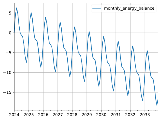
The energy need is the shortfall — the negative part of the monthly energy balance, expressed in average megawatts (aMW). It becomes an input to the model, so we store it as an xarray DataArray.

dummy_energy_needs_df.index.name = "datetime"
dummy_energy_needs_df["energy_needs_aMW"] = (
    -dummy_energy_needs_df.monthly_energy_balance
).clip(lower=0)
energy_needs_xr = xr.DataArray(dummy_energy_needs_df.energy_needs_aMW)

Resource Generation Profiles

Each resource has a normalized generation profile — its output per unit of installed capacity in each month. We make up dummy monthly profiles for wind and solar at three sites (A, B, C).

def generate_resource_profiles(start_year=2024, years=10, noise_level=0.05):
    # Generate a monthly date range
    dates = pd.date_range(start=f"{start_year}-01-01", periods=years * 12, freq="ME")

    # Base profiles for wind and solar resources
    wind_winter_peak = np.array(
        [0.6, 0.55, 0.5, 0.45, 0.4, 0.35, 0.3, 0.25, 0.3, 0.4, 0.5, 0.55]
    )  # Wind peaking in winter
    wind_summer_peak = np.array(
        [0.3, 0.25, 0.3, 0.4, 0.5, 0.55, 0.6, 0.55, 0.5, 0.45, 0.4, 0.35]
    )  # Wind peaking in summer
    solar_base = np.array(
        [0.1, 0.2, 0.4, 0.6, 0.7, 0.9, 0.95, 0.85, 0.6, 0.4, 0.2, 0.1]
    )  # Solar peaking in summer

    # Create dummy profiles with slight variations
    profiles = {}
    for i, location in enumerate(["A", "B", "C"]):
        # Seed a separate generator per location so the profiles stay reproducible
        wind_seed = hash(f"wind_{location}") % (2**32)
        solar_seed = hash(f"solar_{location}") % (2**32)

        wind_rng = np.random.default_rng(wind_seed)
        if i == 0:
            wind_profile = wind_winter_peak + noise_level * wind_rng.standard_normal(12)
        elif i == 1:
            wind_profile = wind_summer_peak + noise_level * wind_rng.standard_normal(12)
        else:
            # Create a mix or a balanced profile as the third option
            wind_profile = 0.5 * (
                wind_winter_peak + wind_summer_peak
            ) + noise_level * wind_rng.standard_normal(12)

        solar_rng = np.random.default_rng(solar_seed)
        solar_profile = solar_base + noise_level * solar_rng.standard_normal(12)

        # Separate generators for the final noise adder
        wind_noise_rng = np.random.default_rng(wind_seed + 1)
        profiles[f"wind_{location}"] = np.tile(
            wind_profile, years
        ) + noise_level * wind_noise_rng.standard_normal(len(dates))

        solar_noise_rng = np.random.default_rng(solar_seed + 1)
        profiles[f"solar_{location}"] = np.tile(
            solar_profile, years
        ) + noise_level * solar_noise_rng.standard_normal(len(dates))

    # Create a DataFrame with the profiles
    df_profiles = pd.DataFrame(data=profiles, index=dates)

    return df_profiles

# Generate the dummy dataset
df_profiles = generate_resource_profiles()

# Plot the profiles for the first 12 months
df_profiles.groupby(df_profiles.index.month).mean().plot()
plt.xlabel("month")
plt.ylabel("normalized generation")
plt.grid()

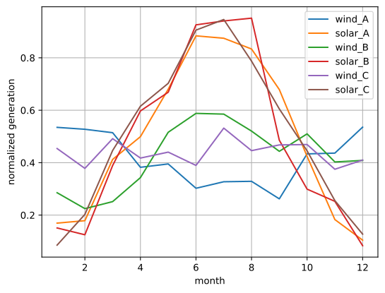
As before, convert to xarray for linopy.

df_profiles.index.name = "datetime"
df_profiles.columns.name = "resource"
resource_profiles_xr = xr.DataArray(df_profiles)

Resource Cost Profiles

Each resource has a unit cost for building capacity. Here the costs decline slowly over time, reflecting technology learning — which gives the model a reason to weigh building sooner against building later.

def generate_unit_cost_profiles(start_year=2024, years=10, decay_rate=0.005):
    # Generate a monthly date range
    dates = pd.date_range(start=f"{start_year}-01-01", periods=years * 12, freq="ME")

    # Initial costs for wind and solar resources
    initial_costs = {
        "wind_A": 1.0,
        "wind_B": 1.2,
        "wind_C": 1.1,
        "solar_A": 0.8,
        "solar_B": 0.85,
        "solar_C": 0.9,
    }

    # Create dummy profiles with slow exponential decay
    profiles = {}
    for resource, initial_cost in initial_costs.items():
        # Exponential decay function
        decay = initial_cost * np.exp(-decay_rate * np.arange(len(dates)))

        # Assign decay curve to profile
        profiles[resource] = decay

    # Create a DataFrame with the profiles
    df_profiles = pd.DataFrame(data=profiles, index=dates)

    return df_profiles


# Generate the dummy dataset
df_unit_cost_profiles = generate_unit_cost_profiles()

# Plot the unit cost profiles
df_unit_cost_profiles.plot()
plt.xlabel("dt")
plt.ylabel("Unit Cost")
plt.legend(title="resource", bbox_to_anchor=(1.05, 1), loc="upper left")
plt.grid()

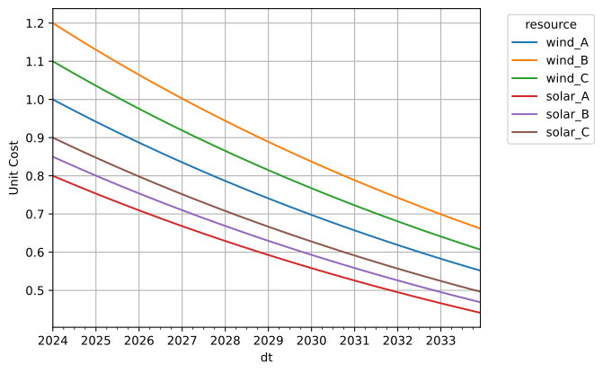
Convert to xarray

df_unit_cost_profiles.index.name = "datetime"
df_unit_cost_profiles.columns.name = "resource"
unit_cost_profiles_xr = xr.DataArray(df_unit_cost_profiles)

Optimized Energy Portfolio Model

With the energy need, generation profiles, and costs in hand, we can write the optimization model. The question it answers is: how much of each resource should we build, and when, to meet the energy need at least cost?

The model has three ingredients, added to an empty linopy.Model across the cells below:

• a decision variable, build_out, holding the installed capacity of each resource in each month,

• constraints that keep the build-out physically sensible and force it to cover the energy need, and

• an objective that minimizes the total build cost.

Because the variable is indexed over both datetime and resource, a single line of linopy expands to a whole array of variables or constraints.

m = lp.Model()

The build-out variable

build_out is the model’s single decision variable, indexed over datetime and resource: build_out[t, r] is the cumulative installed capacity of resource r in month t, bounded below by zero.

Capacity can be added over time but never retired, so the build-out must be non-decreasing: every month must hold at least as much as the month before. build_out.shift(datetime=1) moves the series forward by one month, and the constraint compares each month against its predecessor in a single vectorized call.

Meeting the energy need

Multiplying the availability profiles by the installed capacity gives the generation of each resource in each month; broadcasting over datetime and resource handles the whole grid at once. Summing over resource gives the total generation, which must be at least the energy need in every month.

Cost and objective

Capacity is paid for when it is built, so the cost driver is the capacity added each month — build_out minus the previous month’s value — priced at that month’s unit cost. (In the first month the shift contributes nothing, so the entire initial build-out is charged.) Summing over all months and resources gives the total cost, which becomes the objective to minimize (the default sense of add_objective).

build_out = m.add_variables(
    lower=0,
    dims=resource_profiles_xr.dims,
    coords=resource_profiles_xr.coords,
    name="build_out",
)
m.add_constraints(build_out >= build_out.shift(datetime=1), name="build_out_increasing")

Constraint `build_out_increasing` [datetime: 120, resource: 6]:
---------------------------------------------------------------
[2024-01-31 00:00:00, wind_A]: +1 build_out[2024-01-31 00:00:00, wind_A]                                               ≥ -0.0
[2024-01-31 00:00:00, solar_A]: +1 build_out[2024-01-31 00:00:00, solar_A]                                             ≥ -0.0
[2024-01-31 00:00:00, wind_B]: +1 build_out[2024-01-31 00:00:00, wind_B]                                               ≥ -0.0
[2024-01-31 00:00:00, solar_B]: +1 build_out[2024-01-31 00:00:00, solar_B]                                             ≥ -0.0
[2024-01-31 00:00:00, wind_C]: +1 build_out[2024-01-31 00:00:00, wind_C]                                               ≥ -0.0
[2024-01-31 00:00:00, solar_C]: +1 build_out[2024-01-31 00:00:00, solar_C]                                             ≥ -0.0
[2024-02-29 00:00:00, wind_A]: +1 build_out[2024-02-29 00:00:00, wind_A] - 1 build_out[2024-01-31 00:00:00, wind_A]    ≥ -0.0
                ...
[2033-11-30 00:00:00, solar_C]: +1 build_out[2033-11-30 00:00:00, solar_C] - 1 build_out[2033-10-31 00:00:00, solar_C] ≥ -0.0
[2033-12-31 00:00:00, wind_A]: +1 build_out[2033-12-31 00:00:00, wind_A] - 1 build_out[2033-11-30 00:00:00, wind_A]    ≥ -0.0
[2033-12-31 00:00:00, solar_A]: +1 build_out[2033-12-31 00:00:00, solar_A] - 1 build_out[2033-11-30 00:00:00, solar_A] ≥ -0.0
[2033-12-31 00:00:00, wind_B]: +1 build_out[2033-12-31 00:00:00, wind_B] - 1 build_out[2033-11-30 00:00:00, wind_B]    ≥ -0.0
[2033-12-31 00:00:00, solar_B]: +1 build_out[2033-12-31 00:00:00, solar_B] - 1 build_out[2033-11-30 00:00:00, solar_B] ≥ -0.0
[2033-12-31 00:00:00, wind_C]: +1 build_out[2033-12-31 00:00:00, wind_C] - 1 build_out[2033-11-30 00:00:00, wind_C]    ≥ -0.0
[2033-12-31 00:00:00, solar_C]: +1 build_out[2033-12-31 00:00:00, solar_C] - 1 build_out[2033-11-30 00:00:00, solar_C] ≥ -0.0

gen = resource_profiles_xr * build_out
total_gen = gen.sum(dim="resource")
m.add_constraints(total_gen >= energy_needs_xr, name="meet_energy_need")

Constraint `meet_energy_need` [datetime: 120]:
----------------------------------------------
[2024-01-31 00:00:00]: +0.5256 build_out[2024-01-31 00:00:00, wind_A] + 0.1829 build_out[2024-01-31 00:00:00, solar_A] + 0.2379 build_out[2024-01-31 00:00:00, wind_B] + 0.1998 build_out[2024-01-31 00:00:00, solar_B] + 0.4597 build_out[2024-01-31 00:00:00, wind_C] + 0.04203 build_out[2024-01-31 00:00:00, solar_C]  ≥ -0.0
[2024-02-29 00:00:00]: +0.5604 build_out[2024-02-29 00:00:00, wind_A] + 0.1412 build_out[2024-02-29 00:00:00, solar_A] + 0.1945 build_out[2024-02-29 00:00:00, wind_B] + 0.1128 build_out[2024-02-29 00:00:00, solar_B] + 0.408 build_out[2024-02-29 00:00:00, wind_C] + 0.117 build_out[2024-02-29 00:00:00, solar_C]     ≥ -0.0
[2024-03-31 00:00:00]: +0.5878 build_out[2024-03-31 00:00:00, wind_A] + 0.382 build_out[2024-03-31 00:00:00, solar_A] + 0.2821 build_out[2024-03-31 00:00:00, wind_B] + 0.4034 build_out[2024-03-31 00:00:00, solar_B] + 0.4809 build_out[2024-03-31 00:00:00, wind_C] + 0.4546 build_out[2024-03-31 00:00:00, solar_C]    ≥ -0.0
[2024-04-30 00:00:00]: +0.3457 build_out[2024-04-30 00:00:00, wind_A] + 0.4394 build_out[2024-04-30 00:00:00, solar_A] + 0.3491 build_out[2024-04-30 00:00:00, wind_B] + 0.6568 build_out[2024-04-30 00:00:00, solar_B] + 0.3465 build_out[2024-04-30 00:00:00, wind_C] + 0.6799 build_out[2024-04-30 00:00:00, solar_C]   ≥ -0.0
[2024-05-31 00:00:00]: +0.3817 build_out[2024-05-31 00:00:00, wind_A] + 0.6415 build_out[2024-05-31 00:00:00, solar_A] + 0.573 build_out[2024-05-31 00:00:00, wind_B] + 0.5889 build_out[2024-05-31 00:00:00, solar_B] + 0.3662 build_out[2024-05-31 00:00:00, wind_C] + 0.7274 build_out[2024-05-31 00:00:00, solar_C]    ≥ -0.0
[2024-06-30 00:00:00]: +0.3113 build_out[2024-06-30 00:00:00, wind_A] + 0.9754 build_out[2024-06-30 00:00:00, solar_A] + 0.6472 build_out[2024-06-30 00:00:00, wind_B] + 0.8947 build_out[2024-06-30 00:00:00, solar_B] + 0.4024 build_out[2024-06-30 00:00:00, wind_C] + 0.8964 build_out[2024-06-30 00:00:00, solar_C]   ≥ 0.16506350946109716
[2024-07-31 00:00:00]: +0.3109 build_out[2024-07-31 00:00:00, wind_A] + 0.9113 build_out[2024-07-31 00:00:00, solar_A] + 0.4445 build_out[2024-07-31 00:00:00, wind_B] + 0.9073 build_out[2024-07-31 00:00:00, solar_B] + 0.5221 build_out[2024-07-31 00:00:00, wind_C] + 0.9984 build_out[2024-07-31 00:00:00, solar_C]   ≥ 0.6
                ...
[2033-06-30 00:00:00]: +0.2328 build_out[2033-06-30 00:00:00, wind_A] + 0.7754 build_out[2033-06-30 00:00:00, solar_A] + 0.5314 build_out[2033-06-30 00:00:00, wind_B] + 0.9391 build_out[2033-06-30 00:00:00, solar_B] + 0.3974 build_out[2033-06-30 00:00:00, wind_C] + 0.7928 build_out[2033-06-30 00:00:00, solar_C]   ≥ 10.9650635094611
[2033-07-31 00:00:00]: +0.3376 build_out[2033-07-31 00:00:00, wind_A] + 0.8447 build_out[2033-07-31 00:00:00, solar_A] + 0.5591 build_out[2033-07-31 00:00:00, wind_B] + 0.9749 build_out[2033-07-31 00:00:00, solar_B] + 0.566 build_out[2033-07-31 00:00:00, wind_C] + 0.9292 build_out[2033-07-31 00:00:00, solar_C]    ≥ 11.400000000000002
[2033-08-31 00:00:00]: +0.3017 build_out[2033-08-31 00:00:00, wind_A] + 0.8664 build_out[2033-08-31 00:00:00, solar_A] + 0.4992 build_out[2033-08-31 00:00:00, wind_B] + 0.9739 build_out[2033-08-31 00:00:00, solar_B] + 0.4715 build_out[2033-08-31 00:00:00, wind_C] + 0.7533 build_out[2033-08-31 00:00:00, solar_C]   ≥ 11.834936490538903
[2033-09-30 00:00:00]: +0.2645 build_out[2033-09-30 00:00:00, wind_A] + 0.7166 build_out[2033-09-30 00:00:00, solar_A] + 0.3435 build_out[2033-09-30 00:00:00, wind_B] + 0.4181 build_out[2033-09-30 00:00:00, solar_B] + 0.4333 build_out[2033-09-30 00:00:00, wind_C] + 0.6841 build_out[2033-09-30 00:00:00, solar_C]   ≥ 13.765063509461093
[2033-10-31 00:00:00]: +0.4675 build_out[2033-10-31 00:00:00, wind_A] + 0.4244 build_out[2033-10-31 00:00:00, solar_A] + 0.538 build_out[2033-10-31 00:00:00, wind_B] + 0.2436 build_out[2033-10-31 00:00:00, solar_B] + 0.4632 build_out[2033-10-31 00:00:00, wind_C] + 0.3619 build_out[2033-10-31 00:00:00, solar_C]    ≥ 16.7
[2033-11-30 00:00:00]: +0.4771 build_out[2033-11-30 00:00:00, wind_A] + 0.2275 build_out[2033-11-30 00:00:00, solar_A] + 0.413 build_out[2033-11-30 00:00:00, wind_B] + 0.2374 build_out[2033-11-30 00:00:00, solar_B] + 0.3545 build_out[2033-11-30 00:00:00, wind_C] + 0.2484 build_out[2033-11-30 00:00:00, solar_C]    ≥ 18.29519052838329
[2033-12-31 00:00:00]: +0.5664 build_out[2033-12-31 00:00:00, wind_A] + 0.1801 build_out[2033-12-31 00:00:00, solar_A] + 0.4738 build_out[2033-12-31 00:00:00, wind_B] + 0.03393 build_out[2033-12-31 00:00:00, solar_B] + 0.4232 build_out[2033-12-31 00:00:00, wind_C] + 0.08503 build_out[2033-12-31 00:00:00, solar_C] ≥ 16.5650635094611

build_month = build_out - build_out.shift(datetime=1)
cost = build_month * unit_cost_profiles_xr
total_cost = cost.sum()
total_cost

LinearExpression
----------------
+1 build_out[2024-01-31 00:00:00, wind_A] + 0.8 build_out[2024-01-31 00:00:00, solar_A] + 1.2 build_out[2024-01-31 00:00:00, wind_B] ... -0.6067 build_out[2033-11-30 00:00:00, wind_C] + 0.4964 build_out[2033-12-31 00:00:00, solar_C] - 0.4964 build_out[2033-11-30 00:00:00, solar_C]

m.add_objective(total_cost)
m

Linopy LP model
===============

Variables:
----------
 * build_out (datetime, resource)

Constraints:
------------
 * build_out_increasing (datetime, resource)
 * meet_energy_need (datetime)

Status:
-------
initialized

The solution holds the optimal build_out for every resource and month. Reshaping it into a wide table lets us plot how each resource’s installed capacity grows over time.

Solve

m.solve()

Restricted license - for non-production use only - expires 2027-11-29
Read LP format model from file /tmp/linopy-problem-ctebq02r.lp
Reading time = 0.00 seconds
obj: 840 rows, 720 columns, 2154 nonzeros
Gurobi Optimizer version 13.0.2 build v13.0.2rc1 (linux64 - "Ubuntu 24.04 LTS")

CPU model: AMD EPYC 7R13 Processor, instruction set [SSE2|AVX|AVX2]
Thread count: 1 physical cores, 2 logical processors, using up to 2 threads

Optimize a model with 840 rows, 720 columns and 2154 nonzeros (Min)
Model fingerprint: 0x41a40a28
Model has 720 linear objective coefficients
Coefficient statistics:
  Matrix range     [2e-02, 1e+00]
  Objective range  [2e-03, 7e-01]
  Bounds range     [0e+00, 0e+00]
  RHS range        [1e-01, 2e+01]

Presolve removed 689 rows and 110 columns
Presolve time: 0.01s
Presolved: 151 rows, 610 columns, 4291 nonzeros

Iteration    Objective       Primal Inf.    Dual Inf.      Time
       0   -1.2638421e+31   2.008648e+33   2.527684e+01      0s
     236    3.4912854e+01   0.000000e+00   0.000000e+00      0s

Solved in 236 iterations and 0.02 seconds (0.00 work units)
Optimal objective  3.491285387e+01

('ok', 'optimal')

sol = m.solution

sol_df = (
    sol.to_dataframe()
    .reset_index()
    .pivot_table(values="build_out", columns="resource", index="datetime")
)
sol_df.plot()
plt.grid()
plt.title("Least Cost Energy Portfolio")

Text(0.5, 1.0, 'Least Cost Energy Portfolio')

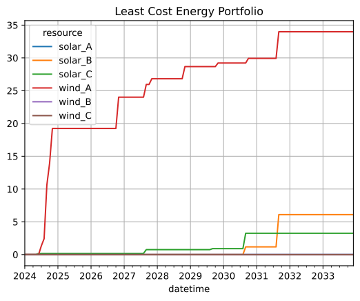
The plot shows the cumulative installed capacity of each resource over time. The lines only ever rise — capacity is added, never retired — and the optimizer meets each month’s energy need with the cheapest combination of resources.

Conclusion

By indexing the variable and constraints over datetime and resource, linopy expresses the whole capacity-expansion problem — hundreds of variables and constraints — in a handful of vectorized lines that mirror how the data is laid out in xarray.